About

Kinda forgot about this site. Bunch of old stuff.
Software Engineer
Kinda forgot about this site. Bunch of old stuff.
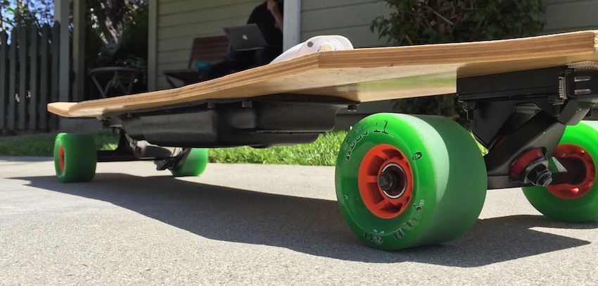
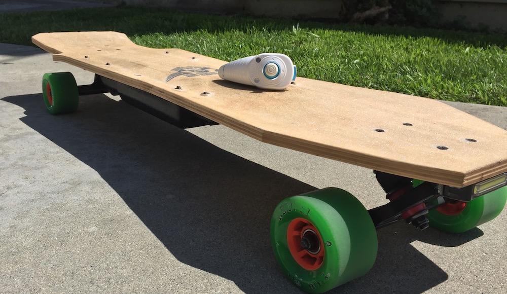
I have always been fascinated with electric vehicles so I decided to build an electric skateboard to improve my commute to school. I started researching for the project in the summer of 2015 and the build begin in early 2016. Although the board is fully operational, I am still adding improvements. The current enhancements include adding a BMS for easier charging/cell balancing and incorporating an iOS app to monitor the speed and various settings for the board. The link below outlines the project from its inception to the current improvements being implemented.
 By Moshanin - https://commons.wikimedia.org/w/index.php?curid=24097346
For a class project I took a crack a classic machine learning algorithm, Collaborative Filtering. The project is designed similar to the “Netflix Prize” competition. Like many collaborative filtering algorithms used in commercial websites and programs, a baseline predictor, user and movie biases, cosine similarity, and nearest neighbor are used to predict user movie ratings. The report used a small sample set the easily demonstrate the core, underlying algorithm.
More Stuff will be added here (lol that was a lie). For now check out my GitHub to find ongoing projects (maybe some super old ones).
I have always had a passion for electric vehicles and with the rise of electric skateboards in particular over the past few years, I figured it would be a great project for an engineering student. For my first build, I planned to use parts that had proven to be effective in the DIY community. Eventually, I hope to use my knowledge from this build along with my schooling to design my own custom motor controller, BMS, remote transmitter, and an iOS application to track and log information.
The board earned the name, ”The Bronco" from an early prototype where eager friends testing it out would unexpectedly be bucked off when the connection from the transmitter to the motor controller would suddenly drop. This can unfortunately be quite a traumatizing experience when traveling at >20mph. These issues have since been fixed and the board is mostly safe for riding today, but it is still important to remember this is not a professional product and can still be incredibly dangerous when reaching high speeds. Overall, the project has proved to be a fun, yet challenging and even frustrating experience at times.

Some nice scuff makes from when the board went rogue and ran into tires and curbs.
This website is new and incomplete. A complete write up is coming soon. Images from the first fully functional design are shown below.
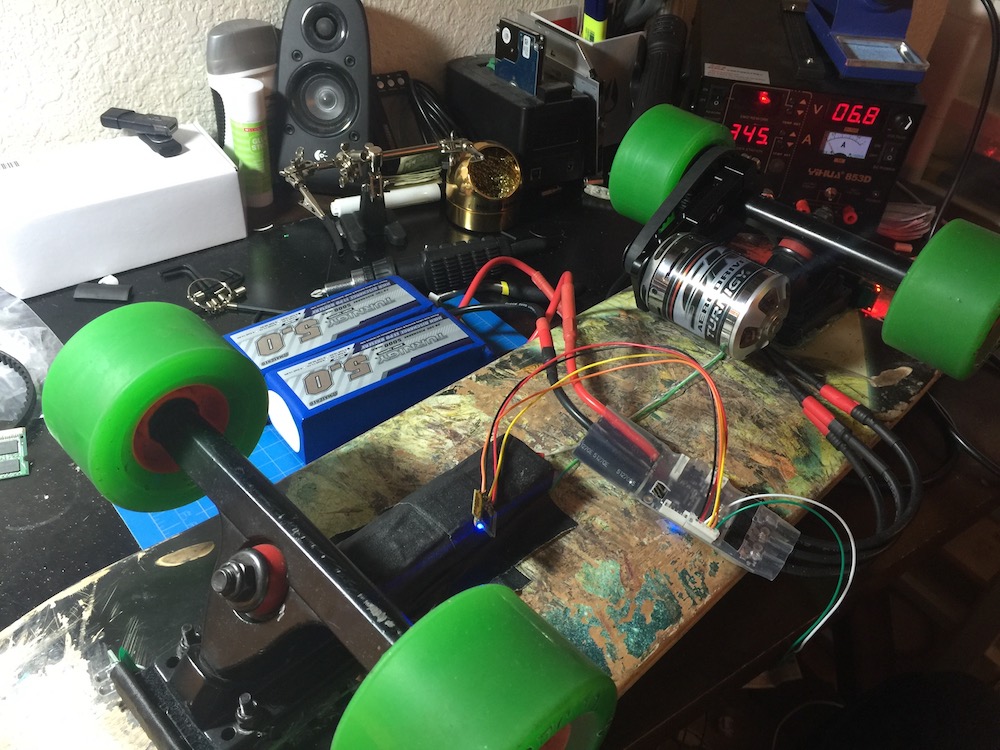
Initial testing
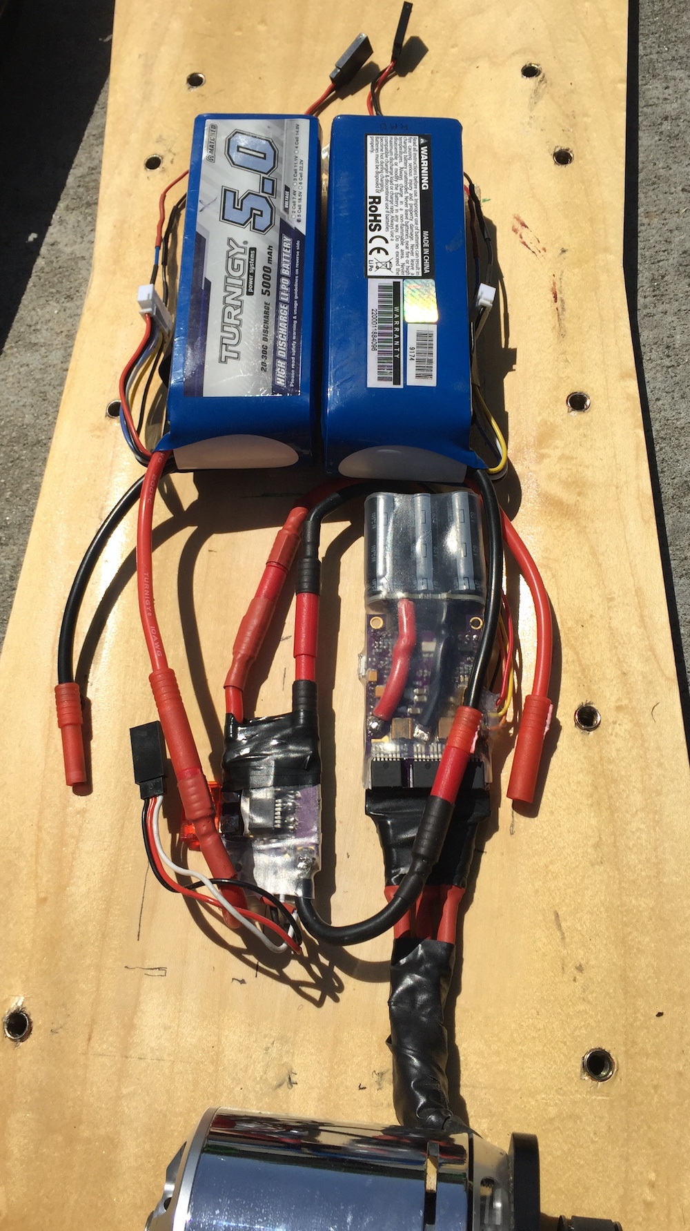
Originally used two 5s 5aH LiPos to power the board. I have since switched to using five 2s 5aH (so the same 10 cell-37V total) for a smaller profile.
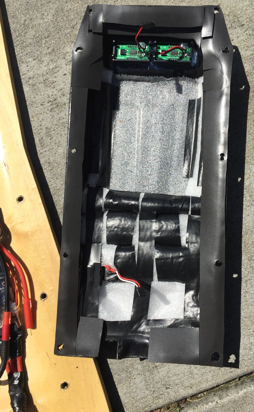
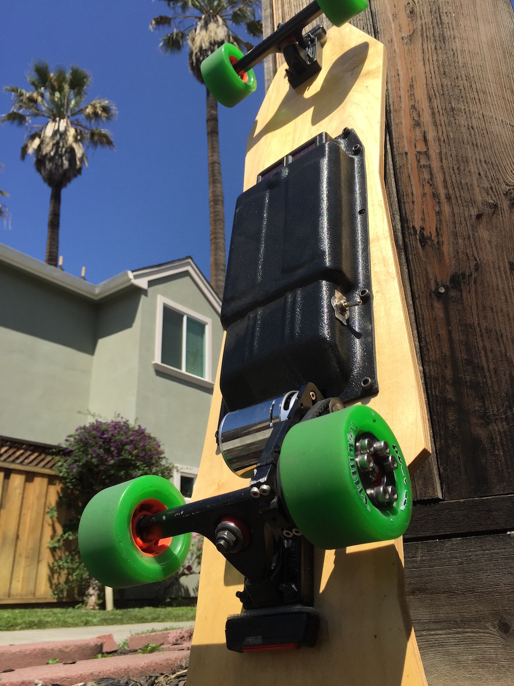
The original enclosure (Flagship V2 by psycotiller). With the new lower profile batteries, a slimmer custom enclosure can be used.
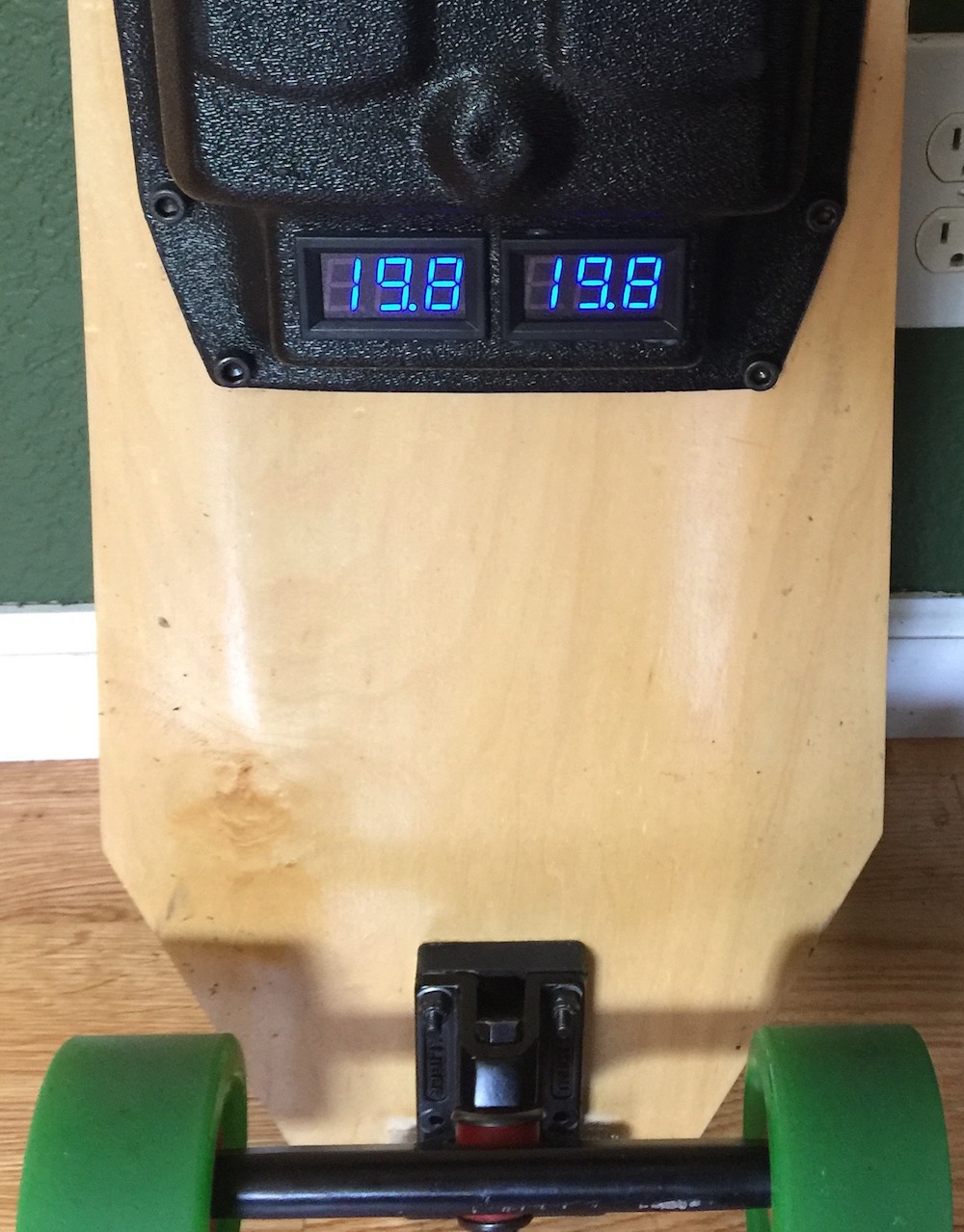
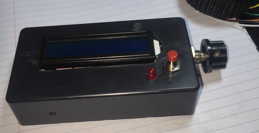
I used a voltmeter to monitor each of the two 5 cell batteries originally, since they kept discharging at different rates.
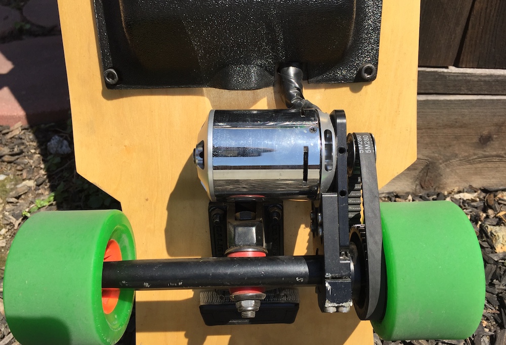
The original drivetrain used a 9mm wide belt at a 16T/36T gearing ratio. I recently switched to a 15mm wide belt which has improved both the acceleration and brake tremendously. The trade off is that it seems to be loosing efficiency. Not a major issue though, since I don't plan on reaching the 30mph speed the board can technically reach at full efficiency.
 By Moshanin - https://commons.wikimedia.org/w/index.php?curid=24097346
This project demonstrates how Collaborative Filtering can predict user ratings of a movie based on other user ratings. The algorithm discussed in this project uses a baseline predictor, user and movie biases, cosine similarity, nearest neighbor predictor, and root mean squared error (RMSE) for evaluating the results. Many commercial implementations will use some variation of these core concepts. The project worked on a small sample set which was able to easily demonstrate the core underlying algorithm.
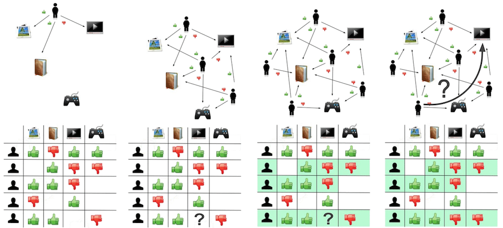
Recommendation engines commonly use collaborative filtering of data from many users to make predictions about a given user’s preferences. The philosophy behind collaborative filtering is that ideal recommendations to a user will come from another user that has similar preferences. These preferences can be calculated by a user rating certain items and creating an estimated representation of that user’s interests. The algorithm would then find similar users that can offer recommendations for an item that the target user has not yet rated.
The gif shown at the top of this page demonstrates how this can be achieved. In this general case the users rate things like books, pictures, games, and videos to create a data set for establishing their preferences. Using collaborative filtering, predictions could then be made for whether or not the target user likes the video. The basis for the predictions is from ratings that similar users rated the target item.

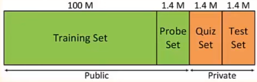
The project follows a scaled down version of the Netflix Prize. It was an open competition to build a collaborative filtering algorithm that could improve their in-house recommendation system for predicting ratings by 10%. Teams were given a data set consisting of a user, their rating for a movie, and the date they rated the movie. However, they were not given anything else pertaining to the user or the films. The algorithms would be tested on a separate set of ratings that were not given to the teams. A grand prize of $1 million was given in 2009 when "BellKor's Pragmatic Chaos" team was able to beat the current prediction algorithm by 10.06%. Their model consisted of a baseline prediction for each user that would take the average of a movie and add a weight to it based on user rating tendencies such as, time of the rating and frequency of ratings. They also used matrix factorization which is used in many collaborative filtering engines. The increased accuracy ended up being too small for justifying the engineering that would be required to implement the winning algorithm in their production environment. Netflix discontinued the competition as lawsuits arose due to insufficient interference control in their datasets allowing users to be identified.
This project took user ratings for various movies and removed some ratings to create a test set to compare against. The algorithm follows a model used by the “Networks Illustrated” course on Coursera by Princeton University.
The prediction engine for this project is written in Python 2.7. It is a simple to read language and allows the functions used to be presented clearly and concisely. Screenshots shown are from the mac OS terminal but any operating system with a Python 2.7 interpreter should be able to recreate the results. The complete source code can be found in the GitHub repository. The equations are displayed on this webpage using MathJax. To format the equations in LaTex so they can be interpreted by MathJax, I used this converter.
In order to create a prediction engine for user ratings of movies, we need data to work with. In this project we will keep it small with just 12 users rating 10 different movies. The reasoning for keeping the set small is to easily illustrate the calculations made at each step in this paper. There are massive datasets available online, such as MovieLens, where some sets contain over 20 million ratings for 27,000 movies by 138,000 users. Problems with these massive sets are that they are incredibly sparse, usually over 99% empty. With the small sample size of this project, we can still accurately demonstrate the core algorithm associated with collaborative filtering in an easy to read manner.
 “Netflix Prize” Networks Illustrated (Brinton,Chaing)
The Netflix Prize data set was removed and only ones left floating around online are extremely outdated with most popular titles not even available anymore. To emulate the same idea as the Netflix Prize, movies were selected from Netflix that were available as of March 2016. The titles chosen were mostly popular titles that received mixed ratings.

As we can see, there is a decent spread in movie genres and years for the small sample size. There was no user in the set who had seen all ten movies and none that had seen less than half
| Title | Genre | Year |
|---|---|---|
| Django Unchained | Drama, Western | 2012 |
| The Interview | Comedy | 2014 |
| The Benchwarmer | Comedy, Sport | 2006 |
| Silver Linings Playbook | Drama, Romance | 2012 |
| Goon | Comedy, Sport | 2011 |
| Pulp Fiction | Crime, Drama | 1994 |
| Days of Thunder | Action, Drama | 1990 |
| Sharknado 3 | Horror, Sci-Fi | 2015 |
| The Lazarus Effect | Horror, Sci-Fi, Thriller | 2015 |
| Grease | Musical, Romance | 1978 |
The user base was built by creating a simple Google Forms survey that listed ten movies with the choices to rate from one to five stars or have not seen. After there were more than 10 responses, I felt there was enough data to work with to make predictions.
The Google Forms automatically creates a spreadsheet that can be saved as a .csv file and accessed by the Python script. The file needed some modification before storing the values as the rows were strings with the number and then “stars” written after. Movies that the user had not seen were given a “-1” value. The code below shows how the values for each rating from the users was extracted from the .csv file.
f = open('/collabFiltering/formResponses.csv')
csvfile = csv.reader(f)
user = [users() for i in range(12)] #list of users
user2 = [users() for i in range(12)] #list of users
index = 0
for row in csvfile:
    user[index].number = index+1
    uRatings = row
    uRatings.pop(0) #pop timestamp off
    for stars in uRatings: #pop "stars" off each
        uStars = stars.replace("stars","")
        uStars = uStars.replace("star","")
        uStars = uStars.replace("Have not seen","-1")
        uStars = uStars.replace(" ","")
        user[index].addRating(int(uStars))
        user2[index].addRating(uStars)
index = index+1Now that all of the data necessary for this project had been obtained, the actual implementation of the collaborative filtering to predict ratings can be designed. This section will walk through each step with the different methods used to achieve the predictions.
Most collaborative filtering algorithms, including the Netflix Prize winner, use a baseline prediction. This is to weight the prediction ratings either higher or lower based on that users ratings tendencies. For example, if they systematically rate movies higher than most other users, then that effect needs to be captured for the final prediction. The equation below shows how the baseline prediction is obtained:
\[b_{u,i}=\mu+b_{u}+b_{i}\]Where \(\mu\) is the overall rating average for that movie, \(b_{u}\) and \(b_{i}\) are the bias values for the user and movie respectively. In simple terms, it is the raw average + user bias + movie bias (the raw average being the mean of all ratings in the matrix). The raw average for the data used in this project is 3.7, calculated in the function raw_average() shown below.
def raw_average(userClass):
	number_of_ratings = 0
	sum = 0
	for i in range(0,len(userClass),1):
		for rating in userClass[i].movie_ratings:
			if (rating>0): # only rated movies
				sum += rating
				number_of_ratings += 1
	return round(float(sum)/float(number_of_ratings),1)
Now to the user and movie bias need to be calculated. The bias will be the average of the ratings (row vector for user, column vector for movies) minus the raw average, as expressed in the equation: \[b_{u}=\frac{1}{\left | I_{u} \right |}\sum_{i\epsilon I_{u}}(r_{u,i}-\mu)\]
The function to implement the user bias is shown below. The function takes in the user number as the parameter and calculates their specific bias. This is the average of the row vector not including the movies that have not been seen.
def user_bias(userNum):
user_obj = user # copy info from getRatings.py
number_of_ratings = 0
sum = 0
for rating in user_obj[userNum].movie_ratings:
	if (rating>0):
		sum += rating
		number_of_ratings += 1
# Subtract raw avg from avg movie score for user
return round(float(sum)/float(number_of_ratings),1)-raw_average(user_obj)
Calculating the movie bias will be very similar, except now it is going to be the average of the column vector minus the raw average. The function movie_bias() below takes a specific movie as the parameter and computes the bias.
def movie_bias(movieNum):
user_obj = user # copy info from getRatings.py
number_of_ratings = 0
sum = 0
# run through each users rating for specific movie
for i in rang(0,len(user_obj),1):
	if (user_obj[i].movie_ratings[movieNum]>0):
		sum += user_obj[i].movie_ratings[movieNum]
		number_of_ratings += 1
return round(float(sum)/float(number_of_ratings),1)-raw_average(user_obj)
With this info, we can now construct a baseline predictor. The bias values computed for users and movies are shown the terminal output below. An example baseline predictor for user 6, movie 3, would be: \[b=3.7+(-0.3)+(-0.6)=2.8\]

This formula can be applied to all values in the user ratings matrix. The baseline predictors for all values is shown in the matrix below.

Although some baselines would come out to be less than 1 or greater than 5, the actual ratings cannot, therefore those values are just given the baselines 1 or 5. To create this bias matrix we can use the code:
bias_obj = [users() for i in range(len(users))]
for j in range(0,len(users),1):
    for i in range(0,len(movies),1):
        rating = round(raw_average(user_obj) + user_bias(j) + movie_bias(i),1)
        if (rating>5.0): #cant have a higher rating than 5
            rating = 5.0
        if (rating< 1.0): #or lower than 1
            rating = 1.0
bias_obj[j].addRating(rating)With the baseline complete, the predictions can be taken a step further by looking at how similar users are to each other. This is really the essence of what collaborative filtering is; searching for patterns in user behavior to enhance the rating estimates. Both strongly positive and negative correlations are helpful. So if two users are somewhat similar or dissimilar, they become neighbors. The patterns for how users rated movies can also be calculated (so it’s not just trying to find patterns on the row vectors, but also on the column vectors).
Cosine similarity was used to compare the users in this data set. Another method, Pearson correlation, is popular in collaborative filtering, but it really only becomes more effective on large, sparse sets (like the MovieLens database). This dataset is small and relatively dense so the cosine similarity will not only be more efficient, but probably more accurate too.
The cosine similarity method takes the normalized dot product of two vectors, which in this algorithm is users and their ratings. An angle of 0 degrees (users rated exactly the same) would produce a value of 1. Similarly, if they are complete opposites producing an angle of 180 degrees, the value will be -1. As mentioned before, this negative correlation is still helpful since we can predict that the users will continue to rate things contradictory.
To implement this design, the equation below shows that the angle is derived by taking the dot product and dividing by the Euclidean norms:
\[s(u,v)=\frac{r_{u}r_{v}}{\left \| r_{u} \right \|\left \| r_{v} \right \|}=\frac{\sum r_{u,i}r_{v,i}}{\sqrt{\sum r^2_{u,i}}\sqrt{\sum r^2_{v,i}}}\]
Vectors that produce values near 0, around a 90 degree angle, will be classified as unknown ratings since they don’t really have a strong correlation to each other. The similarity values are calculated on baseline errors, so the rating predictions are centered at zero to try and correct for errors. To accomplish this, the actual user ratings (from the survey) are subtracted form baseline predictors. This produces a baseline error matrix show below:
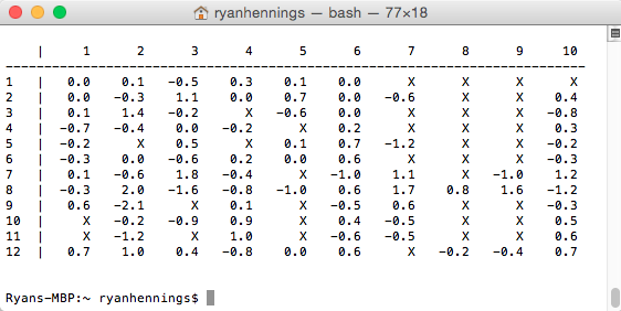
In the baseline error matrix, values of zero indicate zero error, whereas negative values indicate the prediction was too high and vice versa. The values actually entered for movies that have not been seen were 9999 to keep the items in the list same data types. The x’s used in the matrix above are shown for visibility. To create this matrix we can use the code:
baseline_error_obj = [users() for i in range(len(users))]
for j in range(0,len(users),1):
    for i in range(0,len(movies),1):
        if (user_obj[j].movie_ratings[i] < 0):
            err_rating = 9999
        else:
            err_rating = round(user_obj[j].movie_ratings[i] - bias_obj[j].movie_ratings[i],1)
        baseline_error_obj[j].addRating(err_rating)
The equation posted above to achieve this values was implemented in the function userCosineSimilarity() which takes parameters of two lists (the thwo users being compared).
def userCosineSimilarity(user1,user2):
    both_rated = [] # list indices of both rated
    # same vector/user
    if (user1 == user2):
        return 0
    for i in range(0,len(movie_list),1):
        # check for not rated (=9999)
        if (user1[i]< 5.0 and (user2[i]< 5.0))
            both_rated.append(i)

    numerator = 0
    for index in both_rated:
        numerator += user1[index]*user2[index]

    denminator1 = 0
    denminator2 = 0
    for index in both_rated:
        denminator1 += user1[index]*user1[index]
        denminator2 += user2[index]*user2[index]
    denminator = sqrt(denminator1)*sqrt(denminator2)

    return round(numerator/float(denminator),3)
The function returns a number between -1 and 1 rounded to 3 decimal places. Since this function only generates the similarity between two users, the values for all users can be achieved in by simply looping the users through all comparisons as shown below. This is the data used to fill the cosine similarity matrix shown above.
cosine_objs = baseline_error_obj
for i in range(0,len(users),1):
    for j in range(0,len(users),1):
        similarity = userCosineSimilarity(baseline_error_obj[i].movie_ratings, baseline_error_obj[j].movie_ratings)
        cosine_objs[i].addSimilarity(similarity)
For more information on cosine similarity along with other similarity measurement implantations in Python, I found this article helpful.
Now that the similarities between users have been established, each user will choose the user that they are most similar (or dissimilar) to, for predicting their ratings. There are many options on how to implement a nearest neighbor but for this project, a simple brute force method was used to find the person with the highest absolute value. Only one neighbor was used since in this dataset there were only 12 users. If a second neighbor was used in the case that the first could not, they would probably have a low cosine similarity score anyways. Many optimized collaborative filtering algorithms tend to not even use the neighbor if the absolute value of the score is not greater than 0.9.
To find a given users neighbor, you simply traverse down a column or row (since it is a symmetric matrix, the values are the same) of the cosine similarity matrix and find the score closest to the absolute value of 1. We take the absolute value since a strong negative correlation is still helpful. The brute force method to finding the nearest neighbor was implemented with the two functions below:
def nearestNeighbor(userClass):
    maxVal = 0
    for value in userClass.similarity_angle:
        if abs(value) > abs(maxVal):
            maxVal = value
    return maxVal

def nearestNeighborIndex(userNum):
    userIndex = cosine_objs[userNum].similarity_angle.index(nearestNeighbor(cosine_objs[userNum]))
    return userIndex
The nearestNeighbor() function obtains the value of the nearest neighbor for a given user while the nearestNeighborIdex() provides the index at which that value is stored. The index is important because that is the user who the nearest neighbor. The .index function used is predefined in Python and returns the first index for the value being searched. If that value is not preset in the list, the script will halt with an error, but that should never be the case due to the first function always obtaining the cosine similarity value.
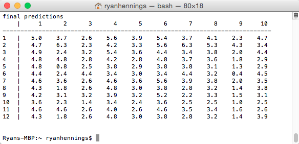
With the neighbors of all of the users found, a final prediction of all the movie ratings can be calculated. Each prediction will be made by taking the baseline prediction used, and adding the error value for produced from the neighbor. It can be easily seen in the equation:
\[FinalPrediction=BaselinePrediction+NeighborErrorPridiction\]
With the help of the code used to create the bias_obj and baseline_error_obj above, we can create the final prediction as follows:
final_predictions = [users() for i in range(len(users))]
for userID in range(0,len(users),1):
    for i in range(0,len(movies),1):
        base_predic = bias_obj[userID].movie_ratings[i]
        neighb = nearestNeighborIndex(userID) #find neighbor
        if (cosine_objs[userID].similarity_angle[neighb] > 0):
            errorRating = baseline_error_obj[neighb].movie_ratings[i]
            if (errorRating < 10): #check for 9999
                final_predictions[userID].addRating(round(base_predic + errorRating, 1))
            else: #neighbor didnt rate movie
                final_predictions[userID].addRating(round(base_predic + 0, 1))

        elif (cosine_objs[userID].similarity_angle[neighb] < 0): #dissimilar
            errorRating = baseline_error_obj[neighb].movie_ratings[i]
            if (errorRating < 10):  # check for 9999
                final_predictions[userID].addRating(round(base_predic + errorRating, 1))
            else:  # neighbor didnt rate movie
                final_predictions[userID].addRating(round(base_predic + 0, 1))
Since some of the error prediction values are negative, this simply means that the predictor was too high and we are going to subtract form the baseline. If the nearest neighbor had not rated the movie, then 0 will be added to the baseline because there is not useful information we can add to the prediction. This is where having multiple neighbors would be useful, as the next neighbor could be checked to see if they had rated the movie. The final predictions using this method can be seen in the terminal output below, with the movies going across from 1 to 10, and the users displayed going down from 1 to 12.
With the predictions finalized, we need a way to evaluate the results. This section will show the statistical analysis of the data along with the algorithm analysis of running and search times.
A common way of measuring the accuracy of recommendation engines in calculating the root mean squared error (RMSE). In simple terms, it indicates how much error is between two datasets. This is the method that was used for the Netflix Prize and will be used to evaluate this project as well. For context, the Netflix Prize winners improved the RMSE of the Netflix in-house algorithm by 10.06%. One of the reasons Netflix used this as the evaluation method is that it places a greater emphasis on large errors. For example, a prediction rating that is 2 stars off, it is penalized 8 times harsher than a prediction rating that is 0.2 stars off. The RMSE takes the sum of the average ratings minus the predicted ratings squared. Then divides this number by the total number of predictions in the dataset and takes the square root of that value. This can be seen more clearly in the equation: \[RMSE=\sqrt{\frac{1}{N}\sum_{N}^{i=1}(x_i-\hat{x_i})^2}\]
This calculation is only performed on the movies that were rated in the dataset since there is no data to compare the predictions to unrated movies. This dataset will be called the training set. Usually there will be a test set, which contains ratings that are not used in building the engine. This can be something as simple as removing a few of the ratings in the training set and then adding them in when calculating the RMSE. The function used to calculate the RMSE is shown in the function calcRMSE()
def calcRMSE(userClass):
    sum = 0
    movies = 0
    for i in range(0,12,1):
        for rating in userClass[i].movie_ratings:
            #ignore movies not rated (-1)
           if (rating > 0):
               diff = rating - raw_average(userClass)
               sum += diff*diff
               movies += 1
    return sqrt((sum/movies))
Using this function, the RMSE can be calculated for each of the datasets
The predictions became more accurate as the criteria for evaluating the prediction increased. To demonstrate the improvements in simple terms, a percentage progression can be shown using the equation: \[(1-\frac{TestingRMSE}{RawAvgRMSE})*100=Percent Improvement\]
Using this shows that the baseline predictor leads to a 6.5% improvement and the neighborhood predictor yields 26.2% improvement. This is a good size improvement for the training data, however, usually a test dataset is used to measure the algorithms accuracy. Creating a test dataset is as simple as removing a few of the ratings taken from the survey and testing the RMSE of their values to the final neighborhood predictor values. This is an aspect of the project that was not thought about beforehand so there was going to be no test data available. Luckily some users from the survey were able to rate some movies after, that they previously had not seen. This turned out to be even more useful since all of their original ratings could be used. The new user ratings were: user 1 rating movie 9 a score of 1, user 7 rating a score of 3, and user 11 rating movies 1 and 9 a score of 4 and 1. The RMSE of these values was 0.5147 for a ridiculous 127% improvement from the raw average. This is an abnormally low RMSE that is almost certainly due to the small sample size. Usually the RMSE of test data like this will actually be a little bit higher than the training set used, since the values in the test set are not included in developing the user/movie biases in the baseline predictions or even the neighbors.
Typical RMSE values for test datasets tend to be in the 0.8 to 0.9 range for professional collaborative filtering algorithms. The Netflix Prize winners boasted an RMSE of just under 0.9 for the test set provided by Netflix.
This project demonstrated a simple collaborative filtering algorithm. The core algorithm discussed, is implemented in many online sites including, but not limited to: Netflix, Amazon, Reddit, Spotify, and Pinterest. It can basically be applied to any to any website in which some item or form of media needs to be recommended to a user. They all will vary in their approach since different goals are needed, but the underlying algorithm discussed in this paper shows how it can be implemented. This section will discuss how different methods could have offered better results in a more optimized fashion.
As mentioned earlier, there are large databases like MovieLens that provide lots of data to test this algorithm on. Choosing to use a small survey as the data seems to be the right approach still, since the goal became to simply describe how collaborative filtering works, as opposed to creating a complete recommendation engine fit for commercial use. The problem with this method however, is that mostly friends and family were used. This could lead to the users rating movies similarly and skewing the results, which was displayed in the test data that had an RMSE value of just over 0.5. If this algorithm was able to achieve that low of an error for the actual Netflix user base, I would probably be the lead engineer of their recommendation team. Realistic errors that they achieve are close to double that of what was calculated in the dataset used for this report. A better scientific approach would have been to survey completely random users of different age groups to make predicting ratings much more difficult.
One of the mistakes with using the movie ratings from the users in the survey was a failure to create a test set. This is important because the accuracy of the algorithm needs to be quantified. For competitions like the Netflix Prize, Netflix did not distribute a certain chunk of ratings from the users so that they could test the RMSE. This would clearly show how well the collaborative filtering was implemented. Luckily, a few results were able to be added to the set after, which is how the final RMSE was calculated for this project. For anyone attempting to recreate this experiment though, it would be recommended to create a test set beforehand.
The movies chosen were also somewhat popular, resulting in users rating most of the movies and doing so similarly. This choice was made intentionally to easily illustrate the numbers being produced, whereas using a large dataset like MovieLens would have mostly empty ratings. There also becomes a problem that some movies can just be hard to predict. This is unofficially known as the "Napoleon Dynamite" problem, as discussed in a New York Times article by Clive Thompson. Users tend to rate movies like this both incredibly inconsistently and unpredictably. Many users love the movie while many hate it and when asked why, they cannot explain it. Entries in the Netflix Prize commonly had over a 15% error for this movie, further proving how tough it is to crack. The movie related to this problem for the dataset in this project was “Sharknado 3”, although it appeared that most users ended up just hating it. Still, two of the four ratings used for the test set were actually for this movie, and the RMSE turned out to be incredibly low. With the small user base and likely similarity between them, this is probably due to random luck.
The path to creating a prediction in this project was a simple one that could have been optimized at just about every step. The first step of creating a baseline prediction is one of the most altered aspects. Many implementations, including the Netflix Prize winners, change the baseline predictions based on when they rated a movie (time changing), and how often a user rated movies (frequency). This step creates a prediction that will already be more accurate before even using other users to adjust the final estimates. Most commercial collaborative filtering algorithms used will incorporate at least these two parameters in developing a baseline.
The next step of defining the similarity between users is where the options grow immensely and there is no specific “right” choice. This project used a Cosine Similarity which is more complicated than a simple Euclidean distance, yet still easy to comprehend and demonstrate in this report. Other common methods used for finding the similarity in users are: the Manhattan distance, which is the sum of the absolute differences of their Cartesian coordinates; the Jaccard similarity, which measures the similarity of two sets by taking the intersection of the sets divided by the union of the sets; and graph based similarity, in which many options including shortest path can be implemented to find similarity. Graph based similarity presents an interesting option as there are so many different ways to optimize it. This could have been an entire report on its own, but the math quickly becomes more complicated and the explanations would have grown even longer in an already extensive write up.
Using the similarity in the predictions could also be modified, as collaborative filtering commonly compares the likeness of items to one another. This project simply showed the similarity between users, but the similarity between the movies is another route that could have been explored and included to help narrow the predictions.
After the similarities are computed, they need to be grouped together. The nearest neighbor method that was implemented also presents many options to optimize the algorithm. A simple brute force method was used that worked fine on the small data set. But this results in running time of \(O(D*N^2)\) where D is the number of users trying to find a neighbor. This is a computation that would much longer on the MovieLens dataset. Different forms of tree algorithms would be recommended for larger sets as the search time could be decreased to a \(O(D*Nlog(N))\) time. Much like with the graph similarities, the nearest neighbor discussion and implementation could easily become a project of its own as there are so many options.
This project went into detail for the underlying algorithm of user based collaborative filtering. It has become an important aspect of machine leaning with the growth of internet information. The ability to recommend products and media to consumers is not only a necessity for earning company’s revenue, but also to just make a program function properly. The ability to successfully acquire useful information from a user’s habits and behaviors is difficult and often overwhelming task. Collaborative filtering offers a solution to this problem by creating recommendations based off other users who exhibit similar behavior.
Back
Adding project details here...
Outline project here...
This is bold and this is strong. This is italic and this is emphasized.
This is superscript text and this is subscript text.
This is underlined and this is code: for (;;) { ... }. Finally, this is a link.
Fringilla nisl. Donec accumsan interdum nisi, quis tincidunt felis sagittis eget tempus euismod. Vestibulum ante ipsum primis in faucibus vestibulum. Blandit adipiscing eu felis iaculis volutpat ac adipiscing accumsan faucibus. Vestibulum ante ipsum primis in faucibus lorem ipsum dolor sit amet nullam adipiscing eu felis.
i = 0;
										while (!deck.isInOrder()) {
										    print 'Iteration ' + i;
										    deck.shuffle();
										    i++;
										}

										print 'It took ' + i + ' iterations to sort the deck.';
| Name | Description | Price |
|---|---|---|
| Item One | Ante turpis integer aliquet porttitor. | 29.99 |
| Item Two | Vis ac commodo adipiscing arcu aliquet. | 19.99 |
| Item Three | Morbi faucibus arcu accumsan lorem. | 29.99 |
| Item Four | Vitae integer tempus condimentum. | 19.99 |
| Item Five | Ante turpis integer aliquet porttitor. | 29.99 |
| 100.00 | ||